From X-ray spectra
to thermal-SZ y

APEC NORMALIZATION

Step 1 · What leaves the X-ray spectral fit?

For one annulus, the standard APEC normalization is

K = 10⁻¹⁴ / [4π D_A²(1+z)²] · ∫ n_en_H dV

The integral is over that annulus's three-dimensional volume. The K used here has already been divided by the annular sky area, in arcmin⁻²: it is a surface normalization, not a total-aperture norm.

APEC → PROJECTED EM

Step 2 · How does K become projected emission measure?

Set dV=Dₐ² dΩ dl and divide the preceding equation by one arcmin². Dₐ² cancels exactly, giving

EM_proj = ∫ n_en_H dl = K_arcmin² · 4π(1+z)² / [10⁻¹⁴ Ω_{1 arcmin²}]

Ω₁arcmin²=(π/10800)²=8.4616e-8 sr. The output EMproj is in cm⁻⁵: a line-of-sight ∫nₑnᴴdl, not a deprojected shell EM.

EM → DENSITY

Step 3 · Use EM to constrain a spherical density

Assume fully ionized cosmic-abundance gas, nₑ=1.2nᴴ, and write

n_e(r) = n₀[1 + (r/r_c)²]^−3β/2,   n_H = n_e/1.2

The line-of-sight integral has an analytic EMproj(R). The calculation area-averages it in each real annulus, then fits n₀, r_c, and β with unweighted log₁₀ EM residuals.

EM_proj(R) = (n₀²/1.2) r_c√π Γ(3β−1/2)/Γ(3β) · [1+(R/r_c)²]^1/2−3β

The current best model is n₀=1.786e-2 cm⁻³, r_c=109.258 kpc, β=0.645088.

The fit RMS is 0.0721 dex and the maximum absolute residual is 0.1336 dex. These are model–data scatter, not error bars.

TEMPERATURE PROXY

Step 4 · How does temperature enter 3-D pressure?

The eight spectral fits give projected kT. To prevent one projected-temperature fluctuation from creating a spurious pressure kink, the y calculation uses only this robust power law:

kT(θ) = 1.148673 · (θ/30′)^-0.200450 keV

Inside 7.91′, T is held at the boundary value (there is no R0–5 spectrum); outside 85.15′ the continuation slope is fixed to 0, so it is again constant. This T(r) is a pressure-projection proxy, not a replacement 3-D spectral fit.

PRESSURE → y

Step 5 · From electron pressure to Compton-y

Electron pressure is Pₑ=nₑkT. The thermal-SZ definition is

y(R) = σ_T/(m_ec²) · ∫_−L^+L n_e(√(R²+l²)) kT(√(R²+l²)) dl

With kT in keV and nₑdl in cm⁻², σT(1 keV)/(mec²)=1.301015e-27 cm² keV⁻¹. The script uses r²=R²+l² and numerically integrates from −L to +L; L=10000′ is a recorded β-model-tail cutoff, not an observed cluster edge.

CUMULATIVE APERTURE

Step 6 · What is cumulative Ycyl?

Integrate y once more in the sky plane:

Y_cyl(5′<θ<Θ) = 2π ∫_5′^Θ y(θ) θ_rad dθ_rad

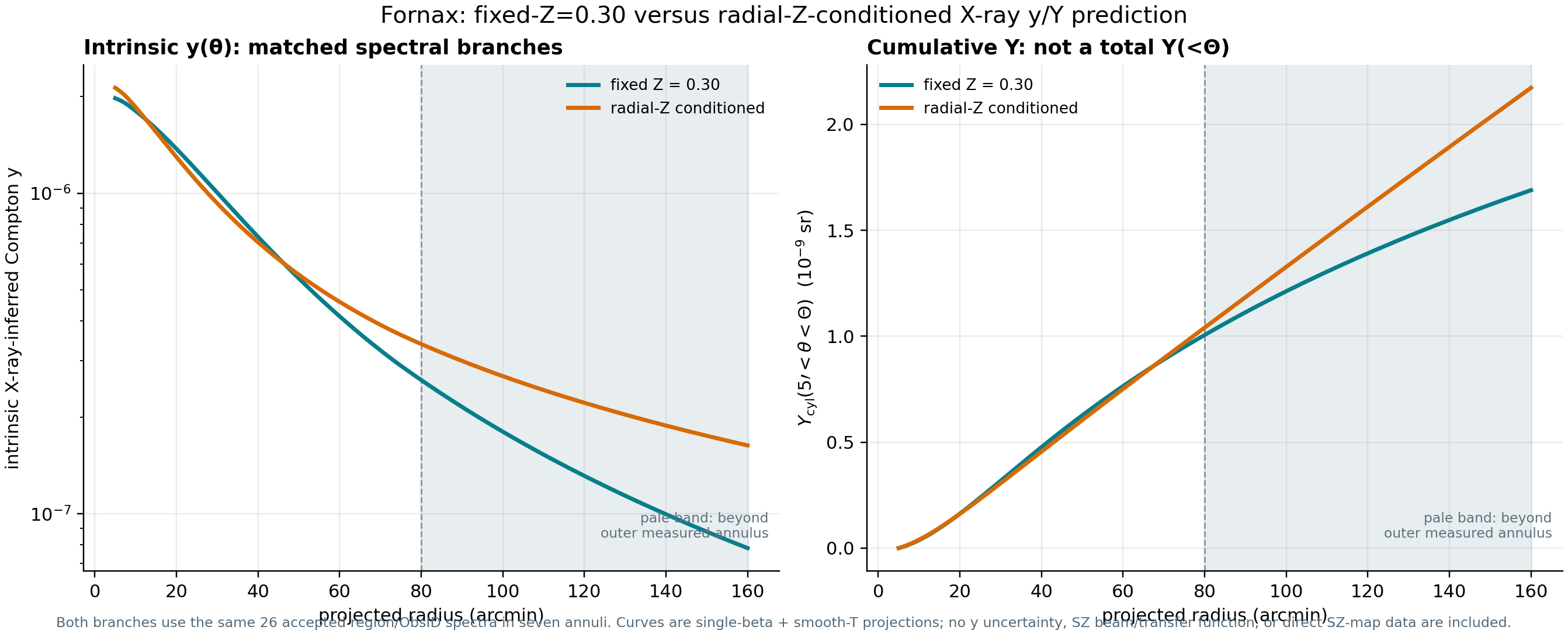
The code computes y on 160 logarithmically spaced radii from 5′ to 180′ and applies the trapezoid rule. Thus it is exactly Ycyl(5′<θ<Θ), not total Y inside Θ: R0–5 is intentionally absent because no retained MOS spectrum exists.